Chapter 1: Vector Analysis

Section 1.1: Vector Operations

Vectors have both direction and magnitude -> need to take both into an account when working with them.
We define four vector operations: addition and three multiplications.

1. Addition of two vectors: tip to tail
   

   \(\overrightarrow{\mathbf{A}} + \overrightarrow{\mathbf{B}} = \overrightarrow{\mathbf{B}} + \overrightarrow{\mathbf{A}}\ (Commutative) \\ \overrightarrow{\mathbf{A}} - \overrightarrow{\mathbf{B}} = \overrightarrow{\mathbf{A}} + \overrightarrow{\mathbf{\textrm{-}B}}\)

2. Multiplication by a scalar: positive scalar a multiplies the magnitude. If a is negative, direction is reversed.
   

   \(a(\overrightarrow{\mathbf{A}} + \overrightarrow{\mathbf{B}}) = a\overrightarrow{\mathbf{A}} + a\overrightarrow{\mathbf{B}}\ (Distributive)\)

3. Dot Product of Two Vectors:
   

   \(\overrightarrow{\mathbf{A}} \cdot \overrightarrow{\mathbf{B}} = AB\cos(\theta) \Longrightarrow Gives\ back\ scalar\ value\ (no\ direction) \\ \overrightarrow{\mathbf{A}} \cdot \overrightarrow{\mathbf{B}} = \overrightarrow{\mathbf{B}} \cdot \overrightarrow{\mathbf{A}}\ (Commutative) \\ \overrightarrow{\mathbf{A}} \cdot (\overrightarrow{\mathbf{B}} + \overrightarrow{\mathbf{C}}) = \overrightarrow{\mathbf{A}} \cdot \overrightarrow{\mathbf{B}} + \overrightarrow{\mathbf{A}} \cdot \overrightarrow{\mathbf{C}}\ (Distributive)\)

4. Cross Product of Two Vectors:
   

   \(\overrightarrow{\mathbf{A}} \times \overrightarrow{\mathbf{B}} = AB\sin(\theta)\hat{\mathbf{n}} \Longrightarrow Gives\ back\ a\ vector \\ \overrightarrow{\mathbf{A}} \times \overrightarrow{\mathbf{B}} = -(\overrightarrow{\mathbf{B}} \times \overrightarrow{\mathbf{A}})\ (Anti\textrm{-}Commutative)\)

Section 1.2: Component Form

An arbitrary vector A can be expanded in terms of basis vectors:

\(\overrightarrow{\mathbf{A}} = A_x\hat{\boldsymbol{\imath}} + A_y{\hat{\boldsymbol{\jmath}}} + A_z{\hat{\boldsymbol{k}}}\)

1. To add vectors, add like components:
   

   \(\overrightarrow{\mathbf{A}} + \overrightarrow{\mathbf{B}} = (A_x + B_x)\hat{\boldsymbol{\imath}} + (A_y + B_y){\hat{\boldsymbol{\jmath}}} + (A_z + B_z){\hat{\boldsymbol{k}}}\)

2. To multiply by a scalar, multiply each component by that scalar:
   

   \(a\overrightarrow{\mathbf{A}} = (aA_x)\hat{\boldsymbol{\imath}} + (aA_y){\hat{\boldsymbol{\jmath}}} + (aA_z){\hat{\boldsymbol{k}}}\)

3. To find dot product, multiply like components then add
   

   \(\overrightarrow{\mathbf{A}} \cdot \overrightarrow{\mathbf{B}} = A_xB_x + A_yB_y + A_zB_z\)

4. To calculate cross product, calculate determinant:
   

   \(\overrightarrow{\mathbf{A}} \times \overrightarrow{\mathbf{B}} = \begin{vmatrix} \hat{\boldsymbol{\imath}} & \hat{\boldsymbol{\jmath}} & \hat{\boldsymbol{k}} \\ A_x & A_y & A_z \\ B_x & B_y & B_z \\ \end{vmatrix} = (A_yB_z - A_zB_y)\hat{\boldsymbol{\imath}} + (A_zB_x - A_xB_z)\hat{\boldsymbol{\jmath}} + (A_xB_y - A_yB_x)\hat{\boldsymbol{k}}\)

Section 1.3: Triple Products

1. Scalar Triple Product: and equivalent expressions
   

   \(\overrightarrow{\mathbf{A}} \cdot (\overrightarrow{\mathbf{B}} \times \overrightarrow{\mathbf{C}}) = \overrightarrow{\mathbf{B}} \cdot (\overrightarrow{\mathbf{C}} \times \overrightarrow{\mathbf{A}}) = \overrightarrow{\mathbf{C}} \cdot (\overrightarrow{\mathbf{A}} \times \overrightarrow{\mathbf{B}})\)

   

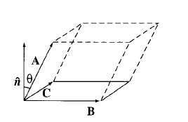
   Geometrically, its absolute value is the volume of a parallelepiped generated by \(\overrightarrow{\mathbf{A}},\ \overrightarrow{\mathbf{B}},\ \overrightarrow{\mathbf{C}}\)

   \(V = Area * Altitude =\left|\overrightarrow{\mathbf{B}} \times \overrightarrow{\mathbf{C}}\right| * A \cos(\theta)\)

   Triple Product expressed in component form:

   \(\overrightarrow{\mathbf{A}} \cdot (\overrightarrow{\mathbf{B}} \times \overrightarrow{\mathbf{C}}) = \begin{vmatrix} A_x & A_y & A_z \\ B_x & B_y & B_z \\ C_x & C_y & C_z \\ \end{vmatrix}\)

   Dot and cross product can be interchanged, but placement of parentheses is critical (cross products are possible only between vectors).

   \(\overrightarrow{\mathbf{A}} \cdot (\overrightarrow{\mathbf{B}} \times \overrightarrow{\mathbf{C}}) = (\overrightarrow{\mathbf{B}} \times \overrightarrow{\mathbf{C}}) \cdot \overrightarrow{\mathbf{A}}\)

2. Vector Triple Product:

   The rule below is known as BAC-CAB rule. It can be used to simplify vector triple products.

   \(\overrightarrow{\mathbf{A}} \times (\overrightarrow{\mathbf{B}} \times \overrightarrow{\mathbf{C}}) = \overrightarrow{\mathbf{B}}(\overrightarrow{\mathbf{A}} \cdot \overrightarrow{\mathbf{C}}) - \overrightarrow{\mathbf{C}}(\overrightarrow{\mathbf{A}} \cdot \overrightarrow{\mathbf{B}})\)

   All higher vector products can be reduced using this rule, so that it is never necessary for an expression to contain more than one cross product in any term.
   For example, these expressions can be simplified (click to see the solution):

   $$(\overrightarrow{\mathbf{A}} \times \overrightarrow{\mathbf{B}}) \cdot (\overrightarrow{\mathbf{C}} \times \overrightarrow{\mathbf{D}}) = (\overrightarrow{\mathbf{A}} \cdot \overrightarrow{\mathbf{C}})(\overrightarrow{\mathbf{B}} \cdot \overrightarrow{\mathbf{D}}) - (\overrightarrow{\mathbf{A}} \cdot \overrightarrow{\mathbf{D}})(\overrightarrow{\mathbf{B}} \cdot \overrightarrow{\mathbf{C}})$$

   $$\overrightarrow{\mathbf{A}} \times (\overrightarrow{\mathbf{B}} \times (\overrightarrow{\mathbf{C}} \times \overrightarrow{\mathbf{D}})) = \overrightarrow{\mathbf{B}}(\overrightarrow{\mathbf{A}} \cdot (\overrightarrow{\mathbf{C}} \times \overrightarrow{\mathbf{D}})) - (\overrightarrow{\mathbf{A}} \cdot \overrightarrow{\mathbf{B}})(\overrightarrow{\mathbf{C}} \times \overrightarrow{\mathbf{D}})$$

Section 1.4: Position, Displacement and Separation Vector

Vector to the point \((x, y, z)\) from the origin is called position vector:

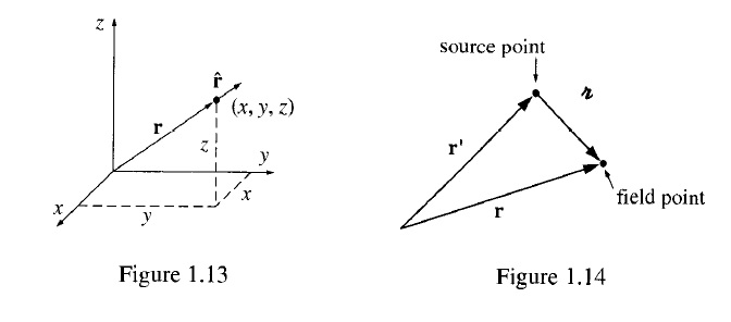
Position Vector: \({\textbf{r}} = {\textit{x}}\hat{\boldsymbol{\imath}} +{\textit{y}}\hat{\boldsymbol{\jmath}} + {\textit{z}}\hat{\boldsymbol{k}}\)
Magnitude: \({\textit{r}} = \sqrt{x^2 + y^2 + z^2}\)

Unit Vector, pointing radially outward in the direction of position vector:. This will make various vector calculus operations a bit easier to understand.

Unit Vector: \(\textit{d}\boldsymbol{l} = \textit{dx}{\hat{\boldsymbol{x}}} + \textit{dy}{\hat{\boldsymbol{y}}} + \textit{dz}{\hat{\boldsymbol{z}}}\)

In E&M, problems frequently deal with two points a source point, \(\textbf{r}\) and field point, \(\textbf{r'}\). Difference between the source point and field point will be called separation vector. Griffith reserves a special symbol for it, script r. I use MathJax javascript library which does not support this character. It will be available in pdf file. Here I will use \(\overrightarrow{\boldsymbol{r}}_{sep}\).

Separation Vector: \(\overrightarrow{\boldsymbol{r}}_{sep}\ = \boldsymbol{r} - \boldsymbol{r'} \)
Unit Vector: \( \hat{\boldsymbol{r}}_{sep}\ =\ \frac{\overrightarrow{\boldsymbol{r}}_{sep}}{\overrightarrow{r}_{sep}}\ =\ \frac{\boldsymbol{r} - \boldsymbol{r'}}{r - r'}\)

In Cartesian coordinates:

Separation Vector: \(\overrightarrow{\boldsymbol{r}}_{sep}\ = (x - x')\hat{\boldsymbol{x}} + (y - y')\hat{\boldsymbol{y}} + (z - z')\hat{\boldsymbol{z}} \)
Magnitude: \(\overrightarrow{r_{sep}}\ = \sqrt{(x - x')^2 + (y - y')^2 + (z - z')^2} \)
Unit Vector: \(\hat{\boldsymbol{r}}_{sep}\ = \frac{(x - x')\hat{\boldsymbol{x}}\ +\ (y - y')\hat{\boldsymbol{y}}\ +\ (z - z')\hat{\boldsymbol{z}}}{\sqrt{(x - x')^2\ +\ (y - y')^2\ +\ (z - z')^2}}\)

Section 1.5: Vector Transformation

Suppose we define a barrel of fruits with pears, apples and bananas \(x,y,z\) like this:

\(Fruit\ Barrel = N_x\hat{\boldsymbol{x}} + N_y\hat{\boldsymbol{y}} + N_z\hat{\boldsymbol{z}}\ where\ N_x,\ N_y,\ N_z\) are quantities of respective fruits.

Q: Is this a vector?

A: No. Although it adds like a vector (we can combine/add barrels together into one bigger barrel, keeping the same structure), it does not transform like a vector. If we reposition the barrel in space or change frame of reference, there is no mathematical formula that can describe proper coordinate transformation, so that we can state that we work with the same barrel.

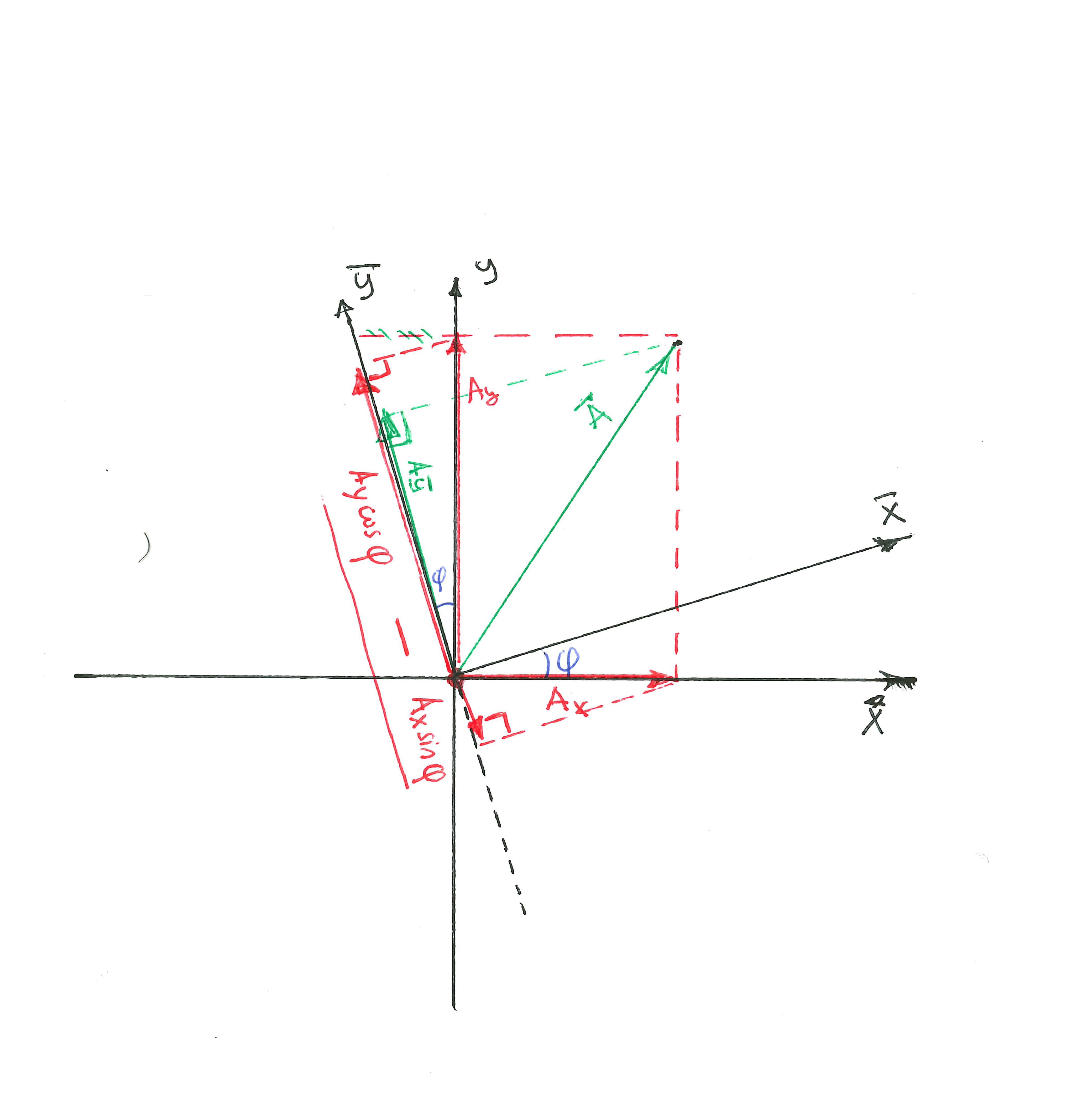
Suppose \(\bar{x},\bar{y},\bar{z}\) is a coordinate system rotated by angle \(\phi\) around \(x\)-axis. Let's take a look at vector A and how it tranforms in this new system.

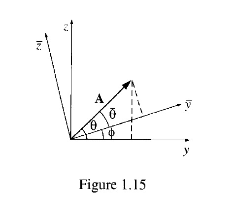
\(\bar{A_y}=A\cos{\bar{\theta}}=A\cos{\theta - \phi}=A(\cos{\theta}\cos{\phi}+\sin{\theta}\sin{\phi})=A_y\cos{\phi}+A_z\sin{\phi} \\ \bar{A_z}=A\sin{\bar{\theta}}=A\cos{\theta - \phi}=A(\sin{\theta}\cos{\phi}+\cos{\theta}\sin{\phi})=-A_z\cos{\phi}-A_y\sin{\phi}\)

This can be written in matrix notation:

$$\begin{pmatrix} \bar{A_y} \\ \bar{A_z} \end{pmatrix} = \begin{pmatrix} \cos{\phi} & \sin{\phi} \\ -\sin{\phi} & \cos{\phi} \\ \end{pmatrix} \begin{pmatrix} A_y \\ A_z \end{pmatrix}$$

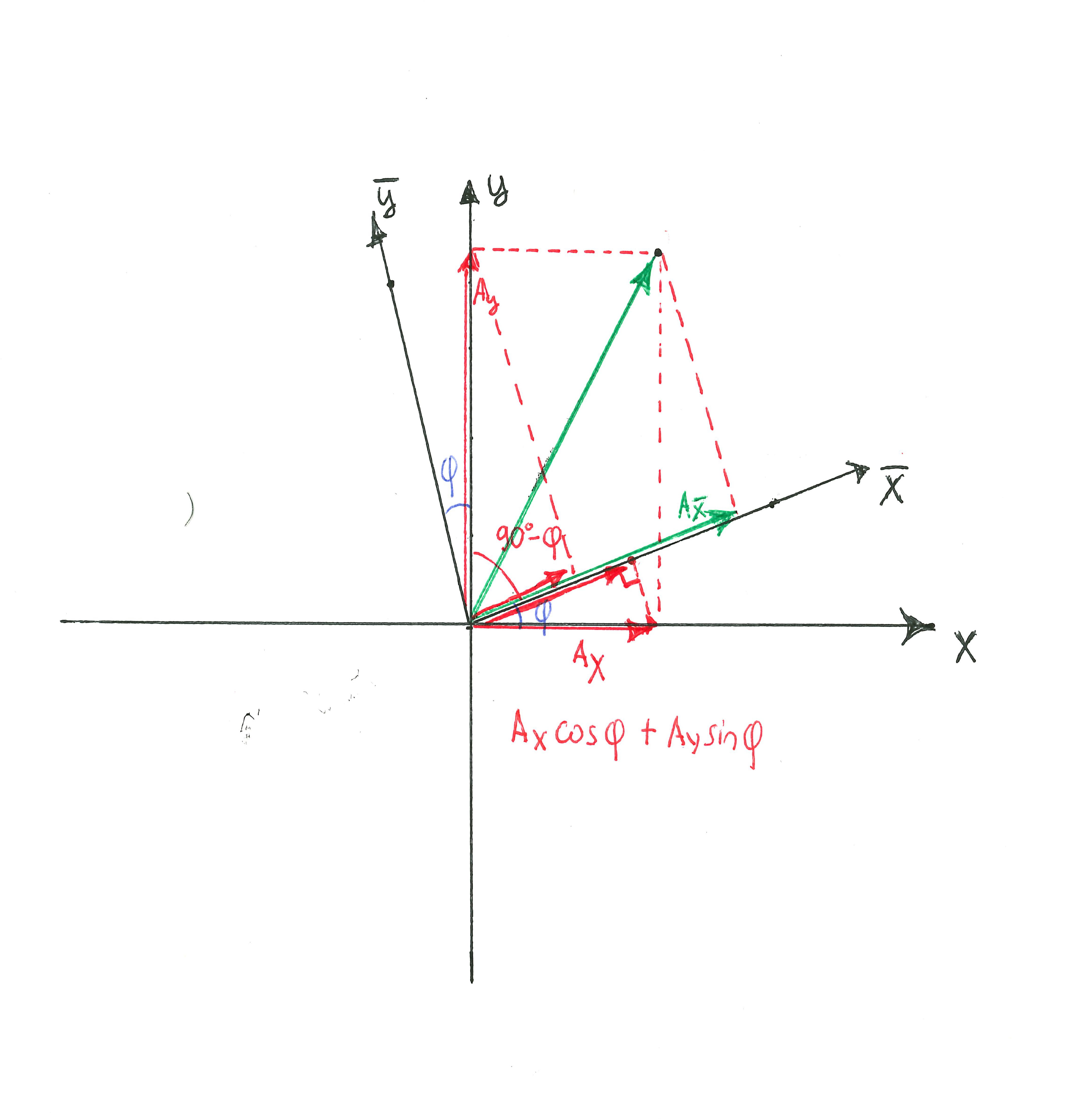
It is easy to see that both vector components in a new set of coordinates are made up of projections of old components along the new set of axes.
\(\bar{A_y} = \underbrace{A_y\cos{\phi}}_\text{\(projection\ of\ A_y\ along\ \bar{A_y}\)} + \underbrace{A_z\sin{\phi}}_\text{\(projection\ of\ A_z\ along\ \bar{A_y}\)} \\ \bar{A_z} = \underbrace{-A_y\sin{\phi}}_\text{\(projection\ of\ A_y\ along\ \bar{A_z}\)} + \underbrace{A_z\cos{\phi}}_\text{\(projection\ of\ A_z\ along\ \bar{A_z}\)}\)

To rotate against an arbitrary axis:

$$\begin{pmatrix} \bar{A_x} \\ \bar{A_y} \\ \bar{A_z} \end{pmatrix} = \begin{pmatrix} R_{xx} & R_{xy} & R_{xz} \\ R_{yx} & R_{yy} & R_{yz} \\ R_{zx} & R_{zy} & R_{zz} \end{pmatrix} \begin{pmatrix} A_x \\ A_y \\ A_z \end{pmatrix} \Longrightarrow \bar{A_i}=\sum_{j=x,y,z}^3 R_{ij}A_j$$

It is evident that similar geometric transformation cannot be applied to barrel of fruits. You can't convert pears into bananas, but you can turn \(A_x\) into \(\bar{A_y}\).

Thus, vector is any set of three components that transforms in the same manner as displacement when you change coordinates. = > displacement as a model for behavior of all vectors.

I choose to omit discussion of tensors because that does not come into play until later chapters.